代码下载
实验目的
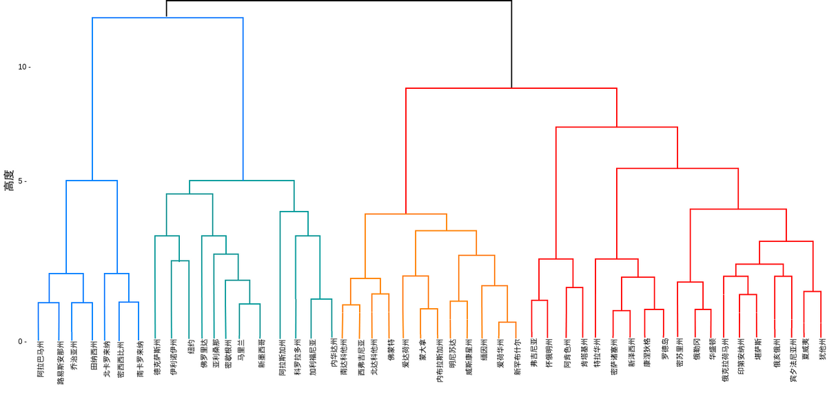
如果您以前从未使用过树状图,那么使用树状图是查看多维数据如何聚集在一起的好方法。 在这本笔记本中,我将简单探索通过层次分析,借助树状图将其可视化。
层次分析
层次分析是聚类分析的一种,scipy有这方面的封装包。
linkage函数从字面意思是链接,层次分析就是不断链接的过程,最终从n条数据,经过不断链接,最终聚合成一类,算法就此停止。
dendrogram是用来绘制树形图的函数。
实验数据
grain_variety是标签,其他列为多种属性的值(特征)。
from scipy.cluster.hierarchy import linkage, dendrogram
import matplotlib.pyplot as plt
import pandas as pd
seeds_df = pd.read_csv('seeds-less-rows.csv')
seeds_df.head()
| area | perimeter | compactness | length | width | asymmetry_coefficient | groove_length | grain_variety | |
|---|---|---|---|---|---|---|---|---|
| 0 | 14.88 | 14.57 | 0.8811 | 5.554 | 3.333 | 1.018 | 4.956 | Kama wheat |
| 1 | 14.69 | 14.49 | 0.8799 | 5.563 | 3.259 | 3.586 | 5.219 | Kama wheat |
| 2 | 14.03 | 14.16 | 0.8796 | 5.438 | 3.201 | 1.717 | 5.001 | Kama wheat |
| 3 | 19.31 | 16.59 | 0.8815 | 6.341 | 3.810 | 3.477 | 6.238 | Rosa wheat |
| 4 | 17.99 | 15.86 | 0.8992 | 5.890 | 3.694 | 2.068 | 5.837 | Rosa wheat |
#移除文本数据列
varieties = list(seeds_df.pop('grain_variety'))
varieties
['Kama wheat',
 'Kama wheat',
 'Kama wheat',
 'Rosa wheat',
 'Rosa wheat',
 'Rosa wheat',
 'Rosa wheat',
 'Rosa wheat',
 'Canadian wheat',
 'Canadian wheat',
 'Canadian wheat',
 'Canadian wheat',
 'Canadian wheat',
 'Canadian wheat']
samples = seeds_df.values
print(samples)
print('samples的维度',samples.shape)
[[14.88   14.57    0.8811  5.554   3.333   1.018   4.956 ]
 [14.69   14.49    0.8799  5.563   3.259   3.586   5.219 ]
 [14.03   14.16    0.8796  5.438   3.201   1.717   5.001 ]
 [19.31   16.59    0.8815  6.341   3.81    3.477   6.238 ]
 [17.99   15.86    0.8992  5.89    3.694   2.068   5.837 ]
 [18.85   16.17    0.9056  6.152   3.806   2.843   6.2   ]
 [19.38   16.72    0.8716  6.303   3.791   3.678   5.965 ]
 [17.36   15.76    0.8785  6.145   3.574   3.526   5.971 ]
 [13.32   13.94    0.8613  5.541   3.073   7.035   5.44  ]
 [11.43   13.13    0.8335  5.176   2.719   2.221   5.132 ]
 [11.26   13.01    0.8355  5.186   2.71    5.335   5.092 ]
 [12.46   13.41    0.8706  5.236   3.017   4.987   5.147 ]
 [11.81   13.45    0.8198  5.413   2.716   4.898   5.352 ]
 [11.23   12.88    0.8511  5.14    2.795   4.325   5.003 ]]
samples的维度 (14, 7)
使用linkage函数对samples进行层次聚类
X = linkage(y, method='single', metric='euclidean')
sacipy中y是距离矩阵,我对此只是傻傻的理解成特征矩阵。 (m*n) m行代表m条记录,n代表n个特征
返回结果X是(m-1)*4的矩阵。 具体含义请看下面的案例
mergings = linkage(samples)

#我们发现mergings比samples少一行
print('sample维度',samples.shape)
print('mergings维度',mergings.shape)
sample维度 (14, 7)
mergings维度 (13, 4)
#层次分析可视化,leaf的字体不旋转,大小为10。
#这里我们不显示每一条数据的具体名字标签(varieties),默认以数字标签显示
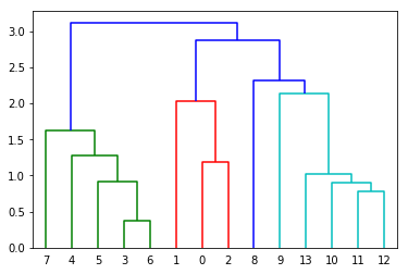
dendrogram(mergings,leaf_rotation=0,leaf_font_size=10)
plt.show()
#在图中显示的数字是最细粒度的叶子,相当于每个样本数据点。
mergings
array([[ 3.        ,  6.        ,  0.37233454,  2.        ],
       [11.        , 12.        ,  0.77366442,  2.        ],
       [10.        , 15.        ,  0.89804259,  3.        ],
       [ 5.        , 14.        ,  0.90978998,  3.        ],
       [13.        , 16.        ,  1.02732924,  4.        ],
       [ 0.        ,  2.        ,  1.18832161,  2.        ],
       [ 4.        , 17.        ,  1.28425969,  4.        ],
       [ 7.        , 20.        ,  1.62187345,  5.        ],
       [ 1.        , 19.        ,  2.02587613,  3.        ],
       [ 9.        , 18.        ,  2.13385537,  5.        ],
       [ 8.        , 23.        ,  2.323123  ,  6.        ],
       [22.        , 24.        ,  2.87625877,  9.        ],
       [21.        , 25.        ,  3.12231564, 14.        ]])
层次分析图从上到下看,依次是枝和叶。
第一列和第二列代表类标签,包含叶子和枝子。
第三列代表叶叶(或叶枝,枝枝)之间的距离
第四列代表该层次类中含有的样本数(记录数)
X = linkage(y, method='single', metric='euclidean')
method是指计算类间距离的方法,比较常用的有3种:
(1)single:最近邻,把类与类间距离最近的作为类间距
(2)average:平均距离,类与类间所有pairs距离的平均
(3)complete:最远邻,把类与类间距离最远的作为类间距
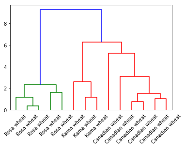
我们写曾侧分析法函数,看看不同的method从图中有什么区别
def hierarchy_analysis(samples,method='single'):
    mergings = linkage(samples, method=method)

    dendrogram(mergings,
              labels=varieties,
              leaf_rotation=45,
              leaf_font_size=10)
    plt.show()
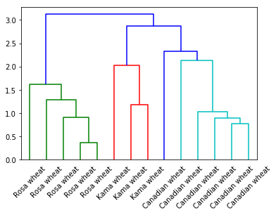
#single
hierarchy_analysis(samples,method='single')
#average
hierarchy_analysis(samples,method='average')
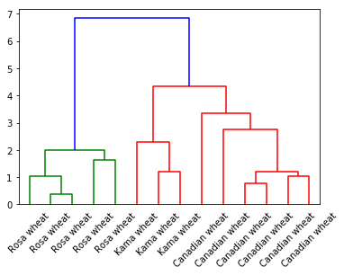
#complete
hierarchy_analysis(samples,method='complete')
由于数据量比较少,complete和average方法做出来的图完全一样。